Proportional Control
Title: Proportional Control Action
Proportional control (P) is one of the most straightforward methods used in control systems. In this method, the controller's output is directly proportional to the error signal between the setpoint and the actual process value. The proportional band typically ranges from 2% to 10%, depending on the application—commonly seen in temperature control systems. However, a key limitation of pure proportional control is that it results in an offset or steady-state error, which is the difference between the setpoint and the actual value after the system stabilizes. To eliminate this error, integral control (I) is often added to the system, ensuring that the long-term error is minimized. The relationship between the proportional band and the controller output is illustrated in the figure below.
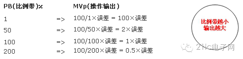
Figure 1

Figure 2: Relationship Between Proportional Band and Output
Steady-State Error (Offset)
In proportional control, when the system reaches a stable state but the error remains non-zero, this residual error is referred to as an offset. This issue occurs because the proportional controller only reacts to the current error, not its duration. As a result, different loads or changes in the system can cause varying levels of offset. The discrepancy between the intersection point of the load curve and the control curve and the desired setpoint is the main cause of this steady-state error. To address this, a manual reset (MR) is often used to adjust the output and reduce the error.

Figure 3: Offset Caused by Proportional Control
Manual Reset

Equation 1: MR – Manual Reset Value
As previously mentioned, proportional control alone cannot eliminate steady-state errors. To compensate for this, a manual reset value (MR) can be adjusted manually to bring the output closer to the desired setpoint. While this method works, it is not practical in real-time applications where frequent adjustments are required. Therefore, integral control is typically introduced to automatically eliminate the offset without human intervention.

Figure 4
Integral Control
Integral Control Action
Integral control (I) is designed to automatically adjust the controller output based on the accumulated error over time. Unlike proportional control, which responds only to the present error, integral control takes into account the history of the error. This allows the system to gradually eliminate the steady-state error. The rate at which the integral action affects the output depends on the integral time setting. The longer the integral time, the slower the response. The goal is to ensure that the controller output eventually matches the desired setpoint.

Figure 5
Definition of Integration Time
The integration time is defined as the time it takes for the integral action to produce the same output as the proportional action would have done if the error had remained constant. This helps determine how aggressively the controller will correct the error over time. A shorter integration time means faster correction, while a longer time leads to a more gradual adjustment.
Differential Control
Differential Control Action (D)
Differential control (D) is used to predict future changes in the error by analyzing the rate of change of the error signal. By anticipating trends, differential control can help stabilize the system and prevent overshooting. It is especially useful when combined with integral control, as it counteracts the potential instability caused by the accumulation of past errors.

Figure 6
Definition of Derivative Time
The derivative time is the time it takes for the differential action to produce the same output as the proportional action would have done if the error were changing at a constant rate. This parameter determines how sensitive the controller is to sudden changes in the error, allowing for more precise and timely adjustments.
Aspheric Lens,Standard Aspheric Lens,Positive Meniscus Lenses,High Precision Aspheric Lens
Danyang Horse Optical Co., Ltd , https://www.dyhorseoptical.com